R Notes

Common R Stuff

Download and Install R Package

install.packages("XML", dependencies = TRUE)

Load a Module

library(XML)

Scrape an HTML Table

library(XML)
u = "http://en.wikipedia.org/wiki/World_population"
# function from XML library, downloads and parses URL for data in HTMLtables
tables = readHtmlTable(u)
names(tables)
tables[[2]]

R Tutorial

Basic R

# x is a vector with values 1 2 3 4 5
x <- 1:5

# create a function
square <- function(x) {
  x^2
}
  
# call fuction with vector x
square(x)

: [1]  1  4  9 16 25

R help

getting help with ?<command-name>

type a ?rnorm, to pop open a manual Page on the R command rnorm
or try ?boxplot to get a help page on the R boxplot function

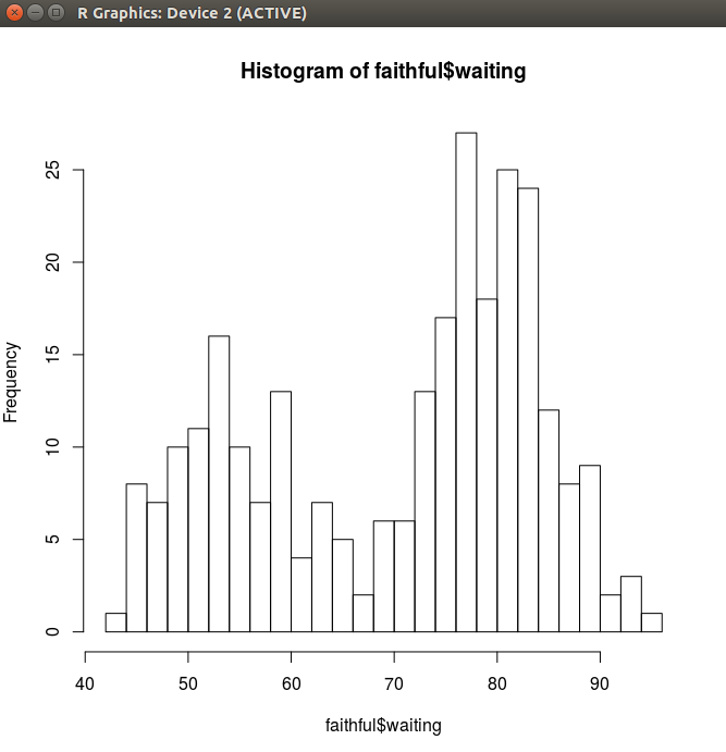
Using Famous Datasets

library(datasets)
data(faithful)
hist(faithful$waiting,breaks=25)

Reading Data into R from Files

dat <- read.table("thedata.txt", sep=":")
# space delimited, also first line is a header
dat2 <- read.table("thedata.txt", header=TRUE)
# csv
dat <- read.csv("thedata.csv")
print(dat)

Reading Data from STDIN

To read data from STDIN, call the scan function with the file parameter left blank
Enter a blank line or Ctrl D to end data input

> nums <- scan()
1: 75  48  61  48 150  49  57  39  27  51  46  50  62  51
15: 
Read 14 items

Reading a Line of Space Separated Data into a vector

```r nums <- scan(textConnection("75 48 61 48 150 49 57 39 27 51 46 50 62 51 50 58 38 34 59 44 24 39 40 33 49 33 34 32 35 30 23 39 36 25 20 32 43 52 42 44 46 51 47 51 44 33 38"), sep=" ") median(nums) mean(nums) deaths <- nums[-5] mean(deaths) median(deaths) sd(deaths) ``` ```r : [1] 44 : [1] 44.93617 : [1] 42.65217 : [1] 43.5 : [1] 11.48761 ```

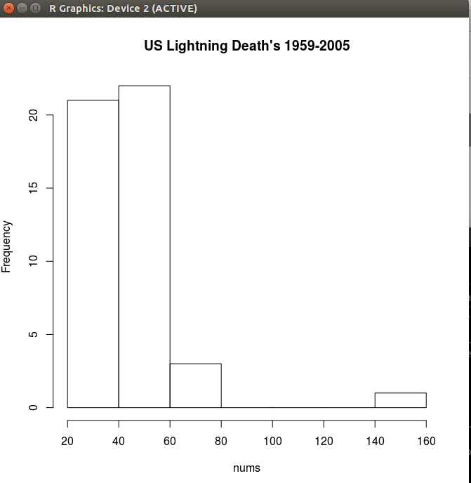
Generating a Histogram

```R # Data pasted from another document can be placed in a vector # via the following composition of functions # textConnection can also be used to read data from stdin nums <- scan(textConnection("75 48 61 48 150 49 57 39 27 51 46 50 62 51 50 58 38 34 59 44 24 39 40 33 49 33 34 32 35 30 23 39 36 25 20 32 43 52 42 44 46 51 47 51 44 33 38"), sep=" ") hist(nums, main="US Lightning Death's 1959-2005") ```

Trimmed Mean to the Rescue

library(datasets)
data(airmiles)
median(airmiles)
# holy right skewed!
mean(airmiles)
# same as median
mean(airmiles,trim=10)
# so its, the top 4% distorting the mean
mean(airmiles,trim=0.4)
#same as median
mean(airmiles,trim=0.5)

: [1] 6431
: [1] 10527.83
: [1] 6431
: [1] 7226.667
: [1] 6431

Drawing a Scatterplot with a Linear Regression line

library(Devore7)
plot(ex12.59)
my.reg <- lm (ex12.59$y ~ ex12.59$x)
abline(my.reg)

Putting 2 plots on 1 image

> par(mfrow=c(2,2))
> boxplot(my.p)
> boxplot(my.h)

Using Reduce and Map

Reduce(f=function,x=vector)

Reduce takes a vector of values, and a binary function and accumulates the values returned over the entire vector of values.

Map(f=function(x){..},x=vector)

Map takes a vector of values and a unary function, runs the function on each value and returns the vector of return values.

here's how to combine them

This function returns the cumulative distribution function of P(x<4) of X~poisson(5).

Reduce("+",Map(function(u){exp(-5)*5^u/factorial(u)},0:3))

: [1] 0.2650259

ANOVA

SSTr - Sum of Square between Treatments

### my.100,m.125,m.150,m.175 are vectors we are analysing
length(m.100)*sum((m.100-mean(m.100))^2)+length(m.125)*sum((m.125-mean(m.125))^2) + length(m.150)*sum((m.150-mean(m.150))^2) + length(m.175)*sum((m.175-mean(m.175))^2)

SSE - Sum of Squares within Treatments

### b.1,b.2, b.3, b.4 are rows of values
### \Sigma (X_{ij} - X_{bar_dot})^2
m.SSE <- sum((b.1-mean(b.1))^2) + sum((b.2-mean(b.2))^2) + sum((b.3-mean(b.3))^2) + sum((b.4-mean(b.4))^2)

Notes on R